Neural Networks for Advertisers
Recently I came across a problem to solve using some sort of machine learning capabilities, which was the need to count the total time during which a specific company was advertised on the various places at a football match.
Not totally sure if this is a real problem or not, I have found it interesting enough to try to solve it with some sort of convolutional neural network architecture and one of the available frameworks like Caffe or Keras and TensorFlow.
The idea is to get the video of the football match, pass it to our deployed neural network, process it and get the total time for which the specified brand was visible to the viewer.
I have revised some pros and cons of different approaches to solve this problem and have chosen one which looks to me like the best in terms of flexibility, speed and complexity.
Possible solutions
Simple OpenCV approach
First approach which came to my mind was to simply solve this problem with OpenCV library itself, assuming I will get promising results using SURF (Speeded-up robust features), which is an improved version of SIFT (Scale Invariant Feature Tranform). In SIFT, Lowe approximated Laplacian of Gaussian with Difference of Gaussian for finding scale-space. SURF goes a little further and approximates LoG with Box Filter.
You can check out an example tutorial for SURF with Python here.
Unfortunately, detecting logos this way quickly turned out almost impossible due to multiple variations of the logo images themselves (logos not fully visible, distorted, rotated etc), not to mention the need to extract the place where the logo is possibly placed using some sort of moving window mechanism.
Image processing and simple single label classification with CNN
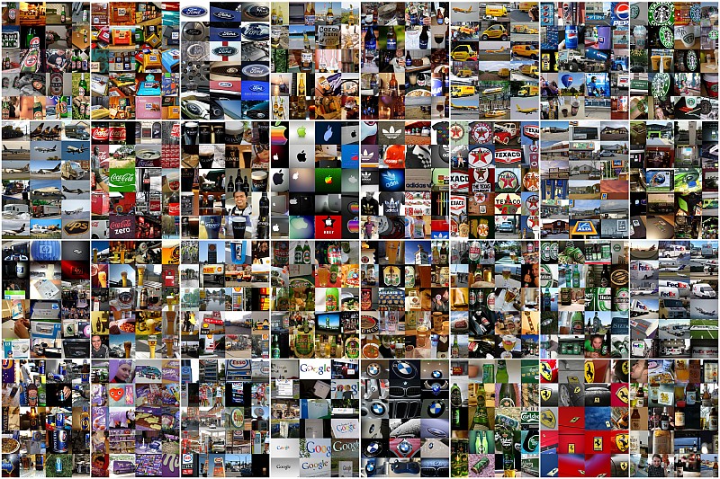
Second solution which could be considered is a kind of brute force approach, where we clip a smaller image from the original and try to classify it with a classifier built using existing datasets available, eg. like the popular dataset from Flickr consisting of 32 logo classes (https://www.uni-augsburg.de/en/fakultaet/fai/informatik/prof/mmc/). The big disadvantage of this approach is that in football match videos, the camera angles and perspectives change in many ways, showing logos in different sizes everywhere on the image frame, and it’s really difficult to find appropriate moving window mechanism which would be reliable enough to retrieve appropriate logo candidates.
CNN multi label classifier
Example CNN architectures useful for multi-label classification are: VGG-16, Inception-v3, ResNet-50
- VGG was originally developed for the ImageNet dataset by the University of Oxford research group. It utilizes 16 layers and 3 x 3 filters in the convolutional layers. It is designed to take in 224 x 224 images as input.
- Inception-v3 is another ImageNet-optimized model. It is developed by Google and it takes in 299 x 299 images.
- ResNet-50 is a model developed by Microsoft Research using a structure that uses residual functions to help add considerable stability to deep networks. ResNet-50 is the 50-layer version of ResNet. It uses 224 x 224 images.
All this networks have a common problem, which is a fixed image size for the input and very long training time. Of course the image size can be modified, but the main issue with this approach is that the predicted classes have to be named upfront and must be a closed set, whereas in the solution described below the training is short and it’s executed separately for each label class.
DetectNet for single/multilabel classification
Some time ago I have read about DetectNet and saw an example run on the DIGITS platform. After a short research, I have convinced myself that it would be a good candidate solution for my problem. All I had to do was to set up appropriate version of DIGITS on Amazon AWS GPU instance and run the Nvidia car object detection example to see what it takes.
According to Nvidia itself:
The use of an FCN within DetectNet is more efficient than using a CNN classifier as a sliding window detector as it avoids redundant computation due to overlapping windows.”
and
On a Titan X GPU using NVIDIA Caffe 0.15.7 and cuDNN RC 5.1 DetectNet can carry out inference on these same 1536×1024 pixel images with a grid spacing of 16 pixels in just 41ms (approximately 24 FPS).”
which looked really promising.
Proof of Concept with DetectNet and DIGITS
DetectNet on DIGITS is best suited to run a single class object detection. At first, it seemed like the wrong way to go, but later I have realized that it would be perfect for a possible real world solution, where we could mix and match different models trained for specific logo brands, and therefore use custom sets of models for some football match we want to get the report on.
The big problem though, with a chosen solution was of course the lack of data. I have quickly realised, after running a few example models for testing purposes, that I would need quite a big dataset to get any usable results after training. While testing DetectNet on DIGITS with different network parameters, bounding boxes data and image sizes I have used a small (about a hundred annotated images) dataset and when I have finally found a setup I wanted to go with, now the only problem left was the proper dataset preparation.
Processed frames are 1248x720 in size and during testing the network setup itself I have found out that approximate numbers for object detection bounding box with DetectNet are 50 to 400 pixel rectangles (those numbers are coming from experience of other users rather than straight calculations), where most of the annotated logo rectangles were around 20-30 pixels in height.
To overcome this problem I have decided to split the images into 4 equal parts and then resize each part to the original image size (therefore quadruple it). This allows me to bring my target objects into the range that DetectNet is sensitive to, but slows down the actual object detection for the full frame 4 times.
It is possible to modify DetectNet settings in such a way that it will work better with smaller objects but simple script for splitting and resizing training data was much faster approach for this Proof of Concept needs.
Dataset preparation
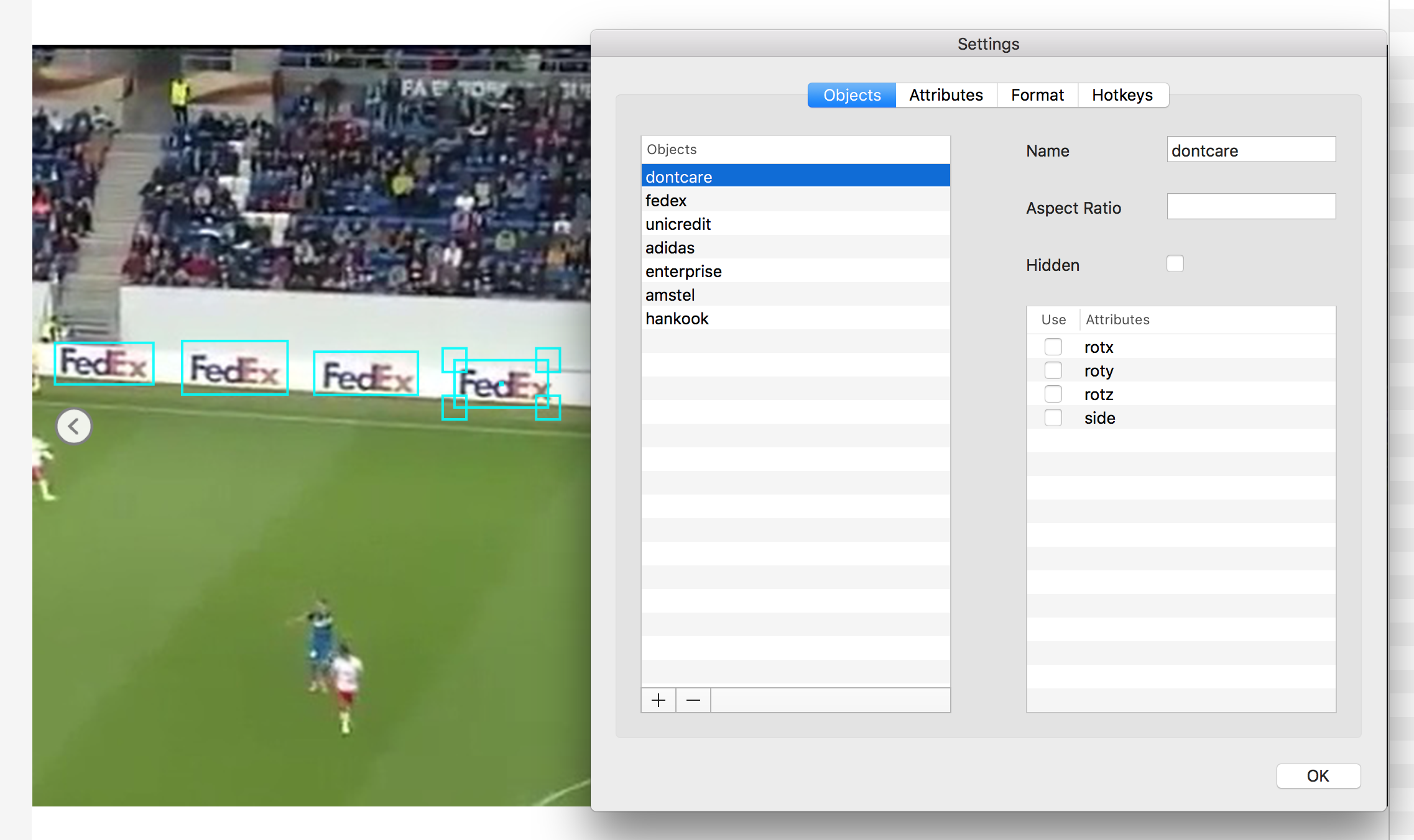
For dataset preparation I have used a freely available software called ‘RectLabel’ from https://rectlabel.com, which has one important property for me - it works on OS X. The software is pretty easy to use, but unfortunately it doesn’t save the data into KITTI format used by DIGITS, for this I had to create a simple converter, which turned out to be pretty easy to do in python.
PASCAL VOC Format:
<annotation>
    <folder>resized</folder>
    <filename>11444_01_02.png</filename>
    <size>
        <width>1280</width>
        <height>720</height>
    </size>
    <segmented>0</segmented>
    <object>
        <name>fedex</name>
        <bndbox>
            <xmin>265</xmin>
            <ymin>665</ymin>
            <xmax>360</xmax>
            <ymax>702</ymax>
        </bndbox>
    </object>
    <object>
        <name>fedex</name>
        <bndbox>
            <xmin>147</xmin>
            <ymin>669</ymin>
            <xmax>237</xmax>
            <ymax>704</ymax>
        </bndbox>
    </object>
</annotation>
KITTI Format:
More information about the KITTI format on Nvidia DIGITS here
fedex 0.00 0 0.00 935 664 1038 711 0.00 0.00 0.00 0.00 0.00 0.00 0.00
fedex 0.00 0 0.00 782 662 896 706 0.00 0.00 0.00 0.00 0.00 0.00 0.00
fedex 0.00 0 0.00 641 662 753 712 0.00 0.00 0.00 0.00 0.00 0.00 0.00
The script for converting the files from one format to the other is pretty easy and can be seen in the project repo. The script itself prepares the data in such a way that it’s ready to be fed into DIGITS - it splits all the annotated files into test and train subsets and creates appropriate directory structure.
def split():
data = numpy.array(os.listdir(sourceDirectory + '/annotations'))
train ,test = train_test_split(data,test_size=0.2)
return train, test
def processSingleFile(filename):
lines = []
if filename.endswith(".xml"):
print("Processing: {0}".format(os.path.join(sourceDirectory + '/annotations', filename)))
e = xml.etree.ElementTree.parse(os.path.join(sourceDirectory + '/annotations', filename)).getroot()
name, xmin, ymin, xmax, ymax = '','','','',''
for elem in e.iterfind('object'):
for oel in elem.iter():
if(oel.tag == 'name'):
name = oel.text.strip()
elif(oel.tag == 'xmin'):
xmin = oel.text.strip()
elif(oel.tag == 'ymin'):
ymin = oel.text.strip()
elif(oel.tag == 'xmax'):
xmax = oel.text.strip()
elif(oel.tag == 'ymax'):
ymax = oel.text.strip()
else:
continue
# Example: Car 0.00 0 3.11 801.18 169.78 848.06 186.03 1.41 1.59 4.01 19.44 1.17 65.54 -2.89
# name 0.00 0 0.00 xmin ymax xmax ymin 0.00 0.00 0.00 0.00 0.00 0.00 0.00
lines.append(name + ' ' + '0.00 0 0.00 ' + xmin + ' ' + ymin + ' ' + xmax + ' ' + ymax + ' 0.00 0.00 0.00 0.00 0.00 0.00 0.00')
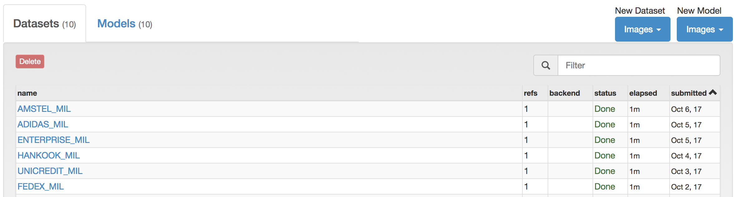
return linesOnce your images are annotated, you can create a dataset for each brand you want to detect. The only difference between datasets on DIGITS is the Custom classes field where you specify the name of the box:
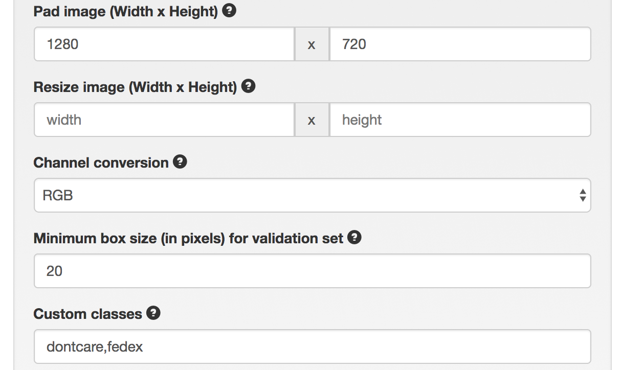
I have created 6 different DIGITS datasets using the same data. All the classes which are not named like the custom class are treated by DIGITS as dontcare.
As you can see from the images below, I had about 1k annotated images and I split them 80/20% for training and testing respectively.
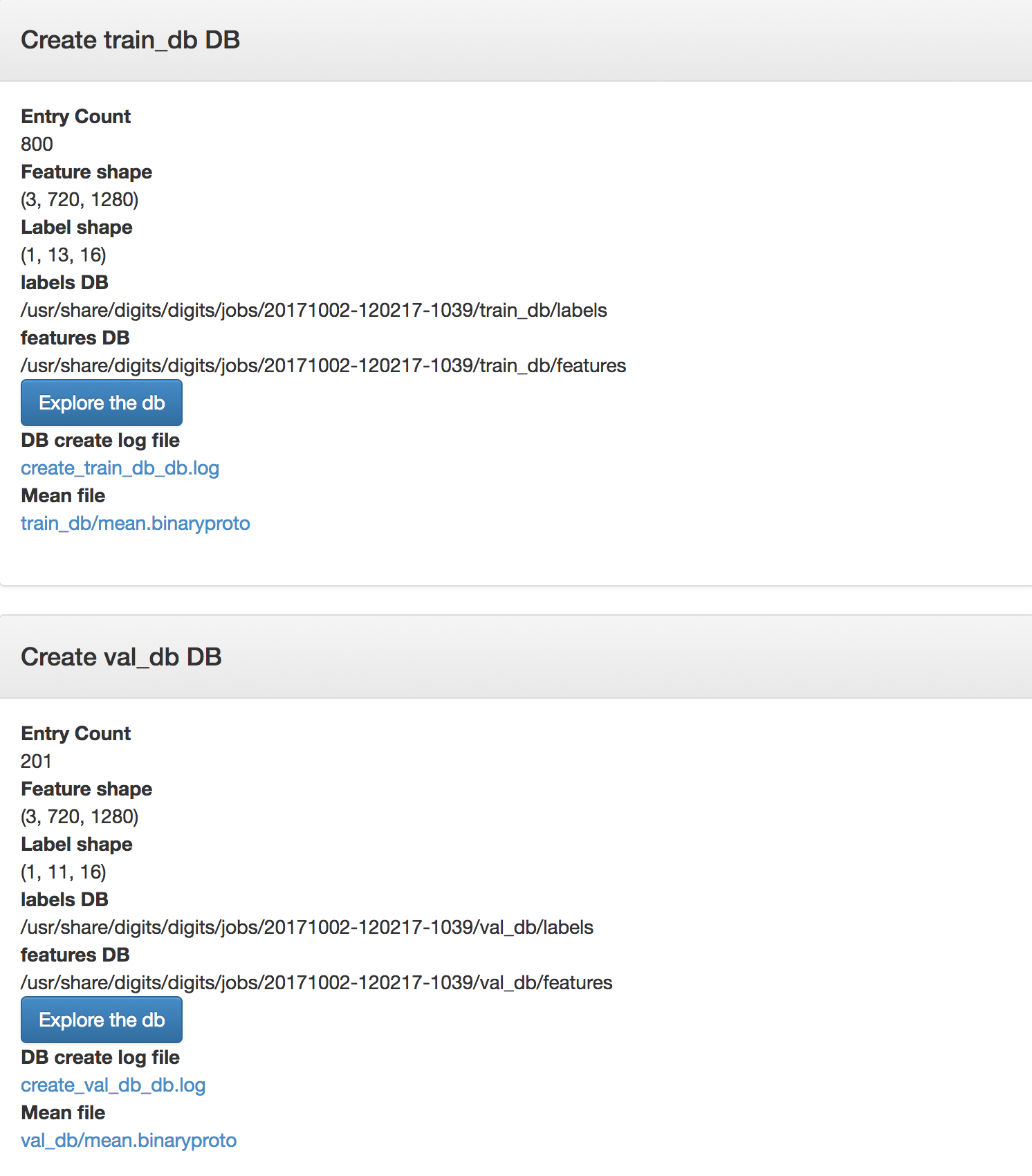
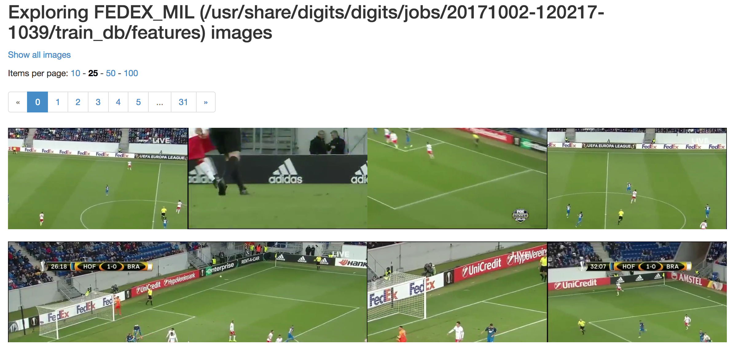
While exploring imported datasets, you can see that the images are enlarged versions of the ¼ of the original video frame.
Training
DetectNet architecture
DetectNet architecture file used for this example (available here) consists of multiple parts like: data input layers definitions, data transformation layers definitions, convolutional network itself, loss layers, mAP calculations and more.
What’s important are the changes made to the data transformation layers, where we specify the image training patch size to be 512x512:
detectnet_groundtruth_param: {
 stride: 16
 scale_cvg: 0.4
 gridbox_type: GRIDBOX_MIN
 coverage_type: RECTANGULAR
 min_cvg_len: 20
 obj_norm: true
 image_size_x: 512
 image_size_y: 512
 crop_bboxes: false
}
which should possibly help detecting smaller objects by taking random crop of this size as input during training every time an image is fed into DetectNet.
Image augmentation parameters were left more or less the same as in the original Nvidia DIGITS Object detection example:
detectnet_augmentation_param: {
    crop_prob: 1
    shift_x: 32
    shift_y: 32
    flip_prob: 0.5
    rotation_prob: 0
    max_rotate_degree: 5
    scale_prob: 0.4
    scale_min: 0.8
    scale_max: 1.2
    hue_rotation_prob: 0.8
    hue_rotation: 30
    desaturation_prob: 0.8
    desaturation_max: 0.8
  }
DetectNet uses combination of two loss functions to calculate the final value used for training optimization (minimized weighted sum of these loss values): bbox_loss and coverage_loss:
# Loss layers
layer {
 name: "bbox_loss"
 type: "L1Loss"
 bottom: "bboxes-obj-masked-norm"
 bottom: "bbox-obj-label-norm"
 top: "loss_bbox"
 loss_weight: 2
 include { phase: TRAIN }
 include { phase: TEST stage: "val" }
}
layer {
 name: "coverage_loss"
 type: "EuclideanLoss"
 bottom: "coverage"
 bottom: "coverage-label"
 top: "loss_coverage"
 include { phase: TRAIN }
 include { phase: TEST stage: "val" }
}
where coverage_loss is the sum of squares of differences between the true and predicted object coverage across all grid squares in a training data sample, and bbox_loss is the mean L1 loss (mean absolute difference) for the true and predicted corners of the bounding box for the object covered by each grid square.
Modified DetectNet (click to enlarge)
The network definition itself can be downloaded from the project repo repo
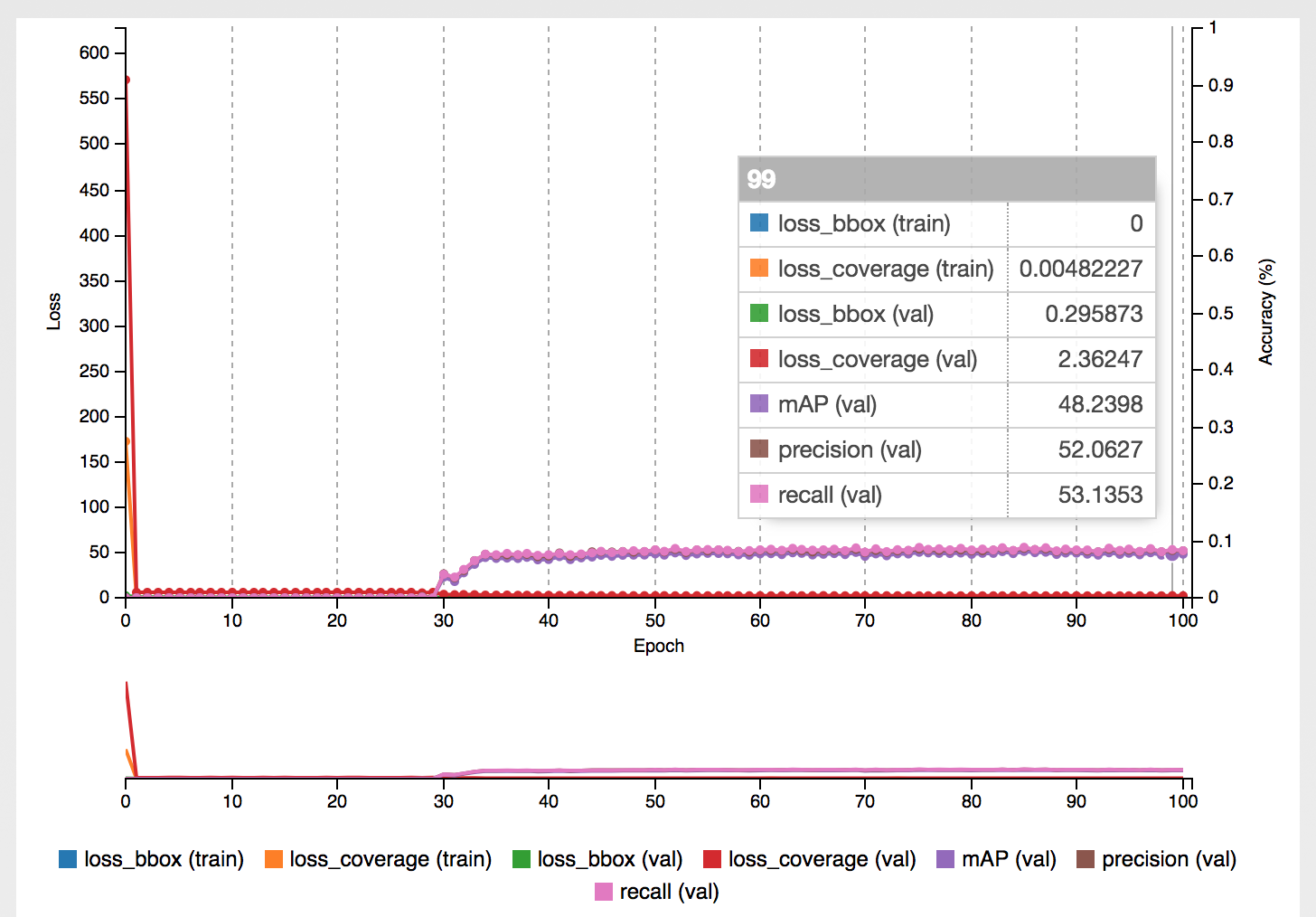
Training outcome
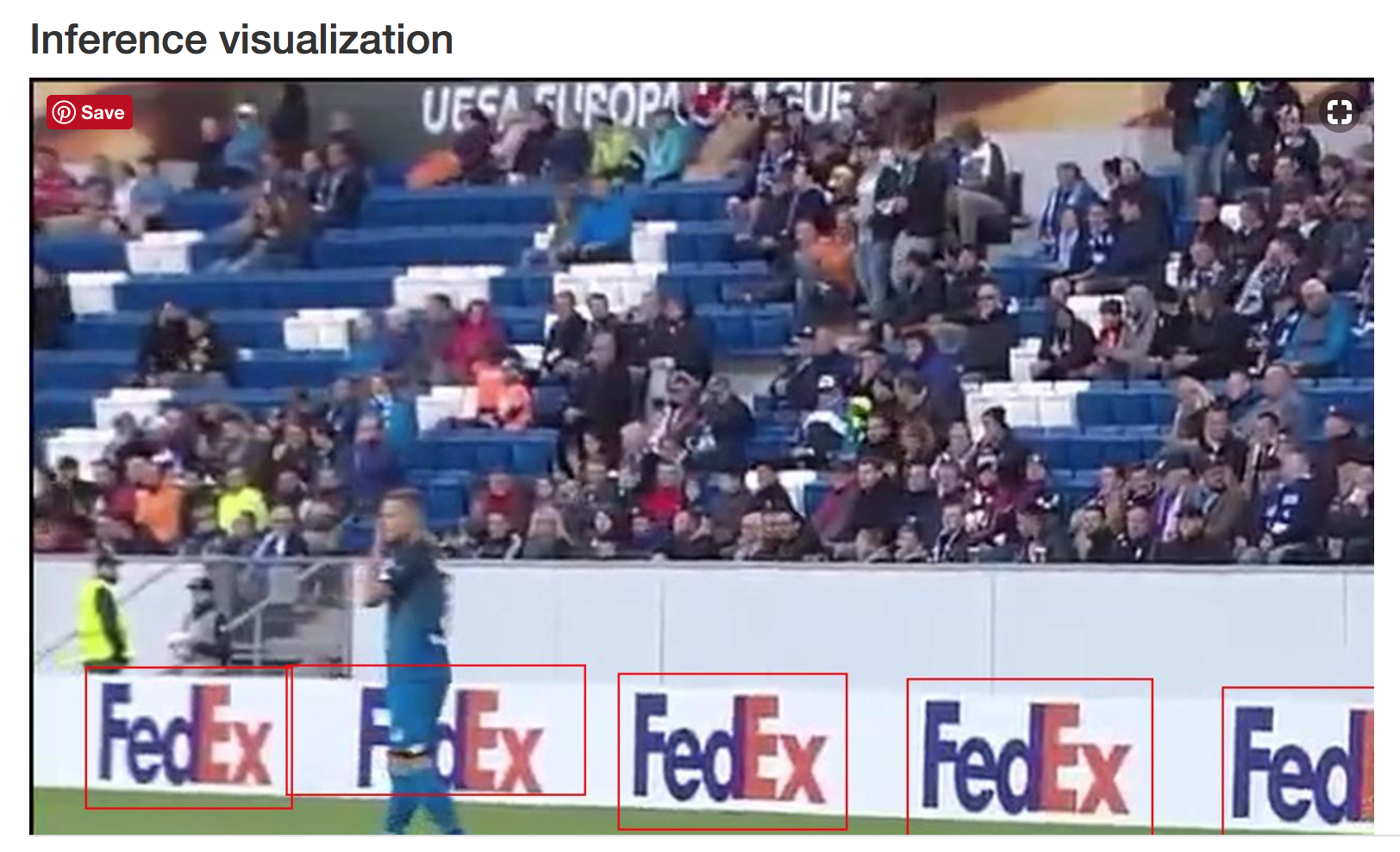
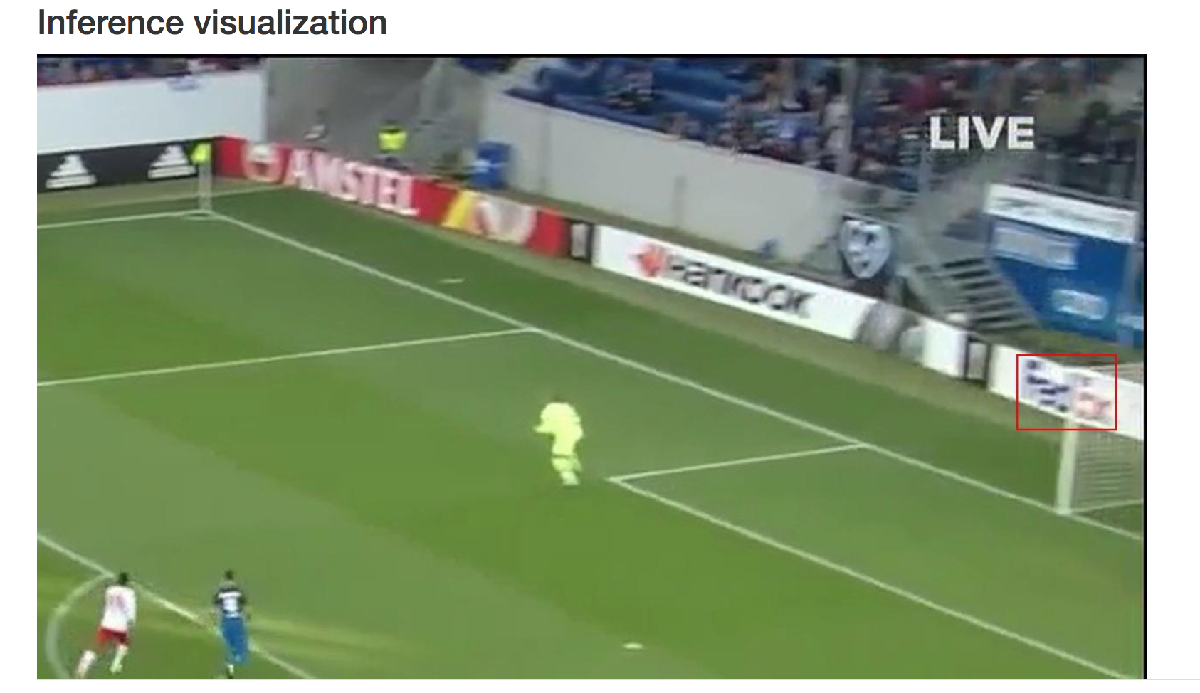
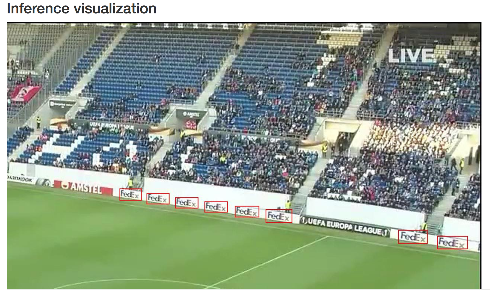
After training the first class for ‘FEDEX’ brand, the model achieved mean average precision of around 67% with precision and recall on validation set at around 72-75%, which for such a small dataset and the POC needs itself was pretty good.
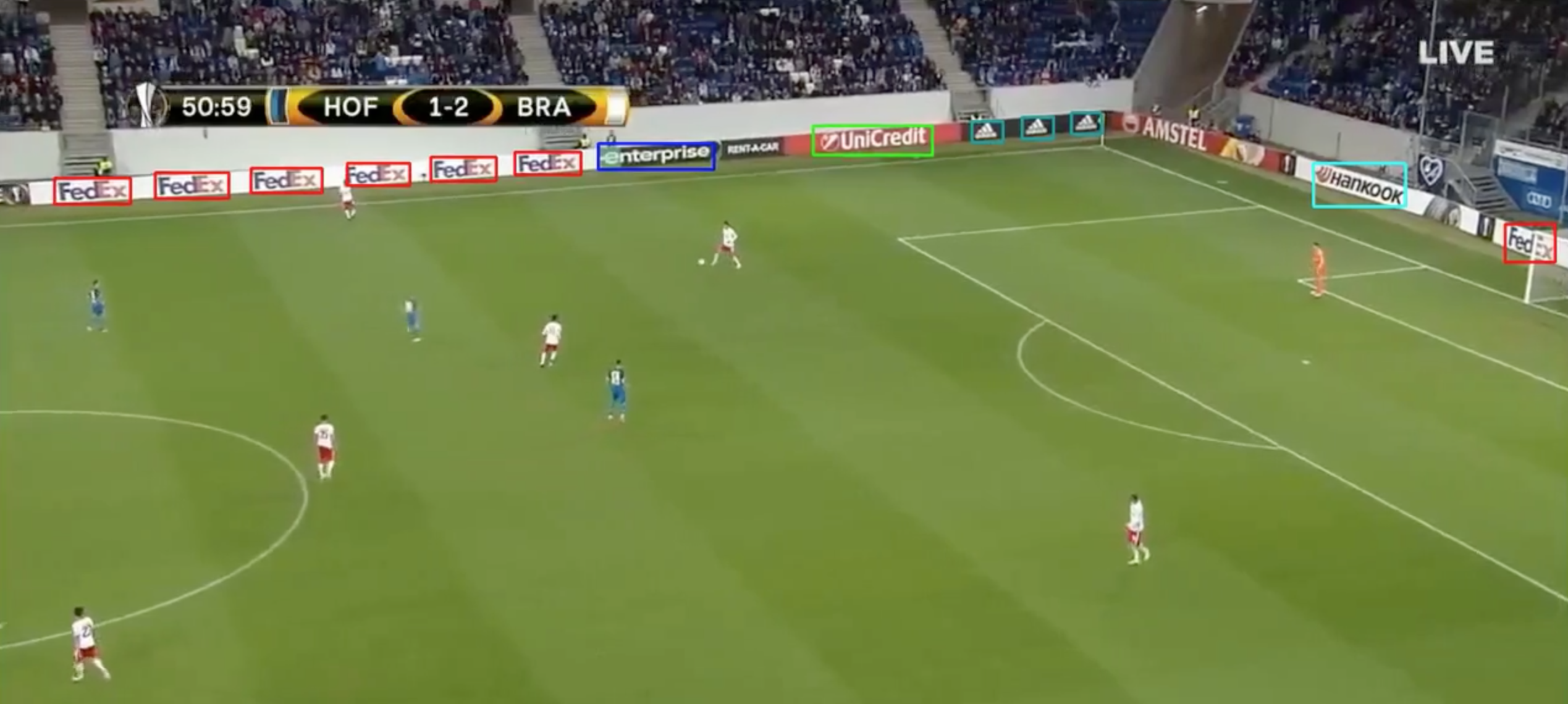
Feeding the DIGITS with example images from the other half of the match shows that the object detections works pretty well:
Other training results:
After annotating 1001 images it turned out that the ‘FEDEX’ was the most often shown brand in the training set, outnumbering the other classes by significant amount.
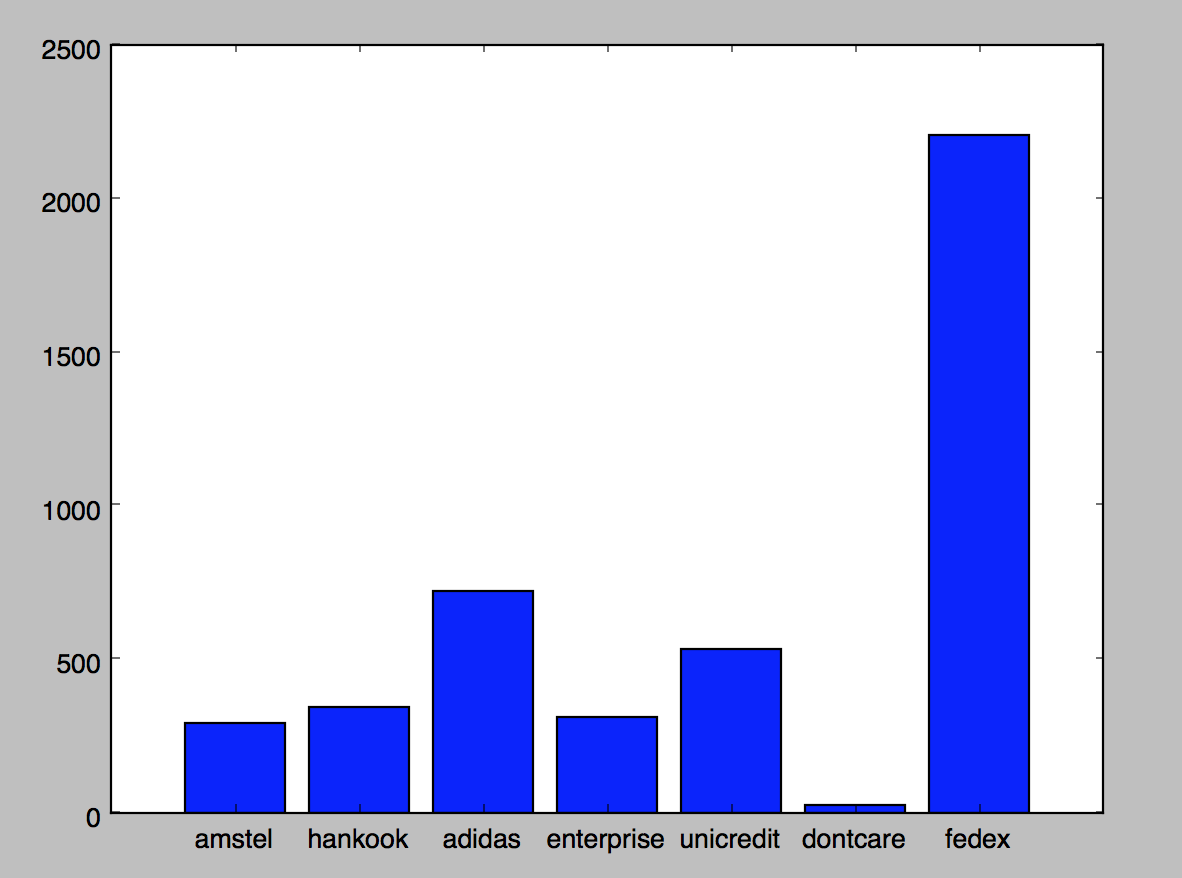
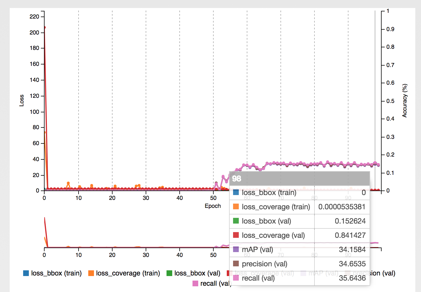
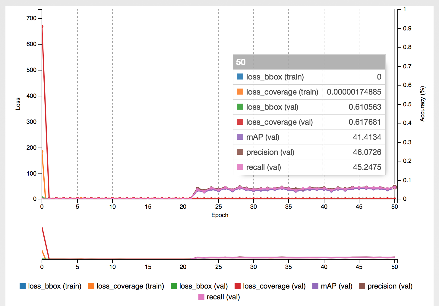
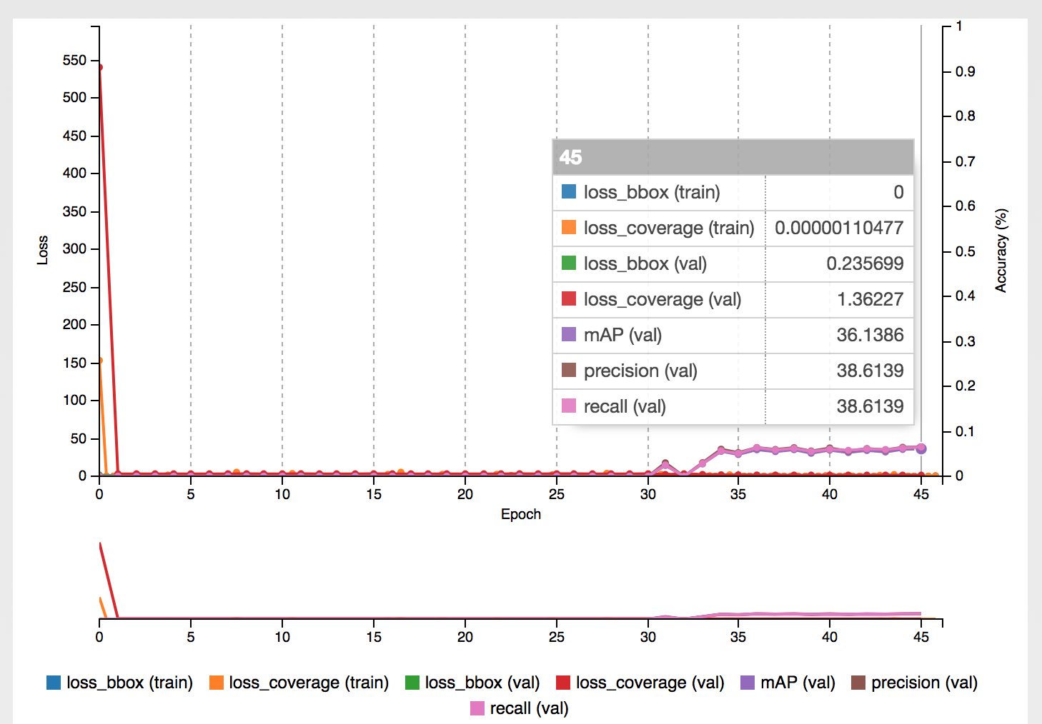
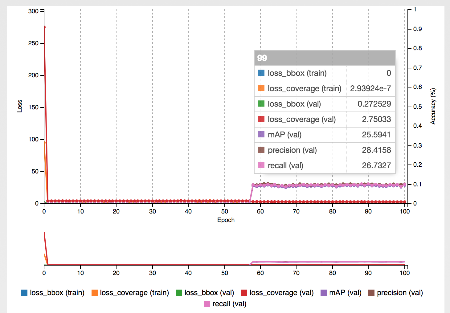
This of course led to poorer results for other classes ranging from 25% mAP for HANKOOK up to 48.5% mAP for UNICREDIT.
AMSTEL
ADIDAS
ENTERPRISE
HANKOOK
UNICREDIT
Real world example
Once the training was done for each class separately, it was time to create a script for the actual processing of the video file and spitting out the results we are most interested in - how long the specific brand was shown on the video.
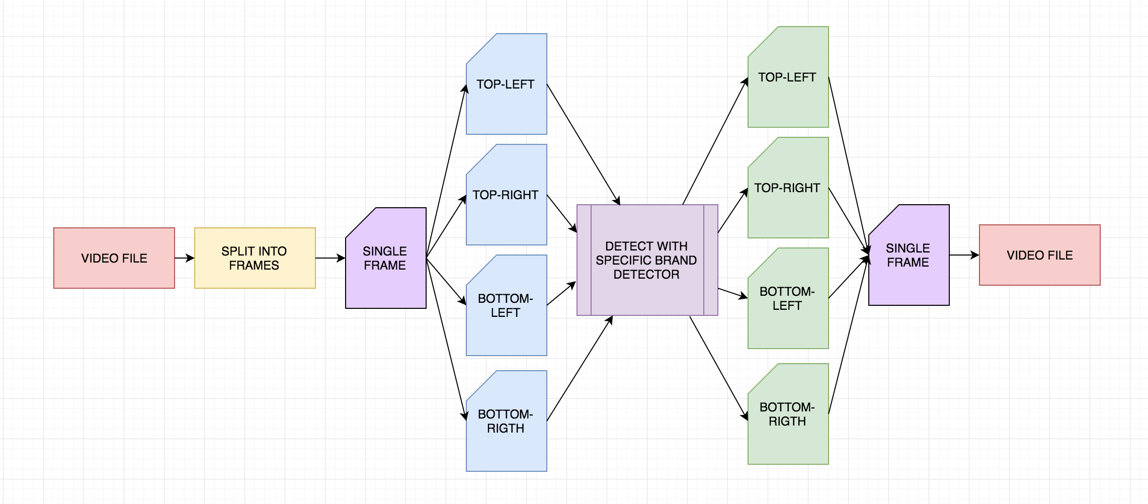
The video file with a football match is read and split into frames using popular python library called moviepy:
clip1 = VideoFileClip(INPUT_FILE)
white_clip = clip1.fl_image(detect_logos_full_img)
white_clip.write_videofile(project_output, audio=True)
detect_logos_full_img is the function which starts the object detection mechanism for each frame.
Once the single frame is obtained from the video, we split it into 4 different images with popular image_slicer python library:
def detect_logos_full_img(image):
    """
    Splits a single frame into 4 images

    Arguments:
    image -- cv2 image file for single video frame
    """
    tiles = slice_image(image, 4)
    modified_images = []
    fullImageBoxes = []
    for i, tile in enumerate(tiles):
        open_cv_image = numpy.array(tile.image)
        image = open_cv_image[:, :, ::-1].copy()
        boxes, img_detected = detect_logos(image)
        modified_images.append(toPILImage(img_detected))
        fullImageBoxes.append(boxes)
    img = joinImages(modified_images)
    allBoxes = merge_dicts(fullImageBoxes)
    addLogoEntry(Logo(frameNumber, allBoxes))
    incrementFrameNumber()
    return toOpenCVFormat(img)
and run the object detection for each image separately (detect_logos(image) function).
Because the image_slicer library uses PIL under the hood, and for most of our work we use OpenCV Image instance, we need to convert the images from one format to the other.
detect_logos function executes the object detection for each model and draws appropriate bounding boxes in different colors onto the image:
def detect_logos(image):
    """
    Runs our pipeline given a single image and returns another one with the bounding boxes drawn

    Arguments:
    image -- cv2 image file being 1/4 of the original
    """
    result = image
    boxes = {}
    for model in MODELS:
        print("Detecting bboxes for: " + model)
        clr = getColorForClass(model)
        boxesFound, result = classify('./models/'+model+'.caffemodel', DEPLOY_FILE, result, clr, MEAN_FILE, BATCH_SIZE, USE_GPU)
        boxes[model] = boxesFound
    return (boxes, result)
It returns the dictionary of found bounding boxes for each class used later for statistics.classify method is the heart of object detection with trained caffe model - it takes an image and executes a forward pass on the trained model to get the information about bounding boxes found. Found bbox information is then used to draw rectangles in specific places in the image.
After the images are processed through all the trained models and all the bounding boxes are drawn, they are merged back into a single image with joinImages function:
def joinImages(modified_images):
result = Image.new("RGB", (1280, 720))
for index, img in enumerate(modified_images):
img.thumbnail((640, 360), Image.ANTIALIAS)
result.paste(modified_images[0], (0, 0))
result.paste(modified_images[2], (0, 360))
result.paste(modified_images[1], (640, 0))
result.paste(modified_images[3], (640, 360))
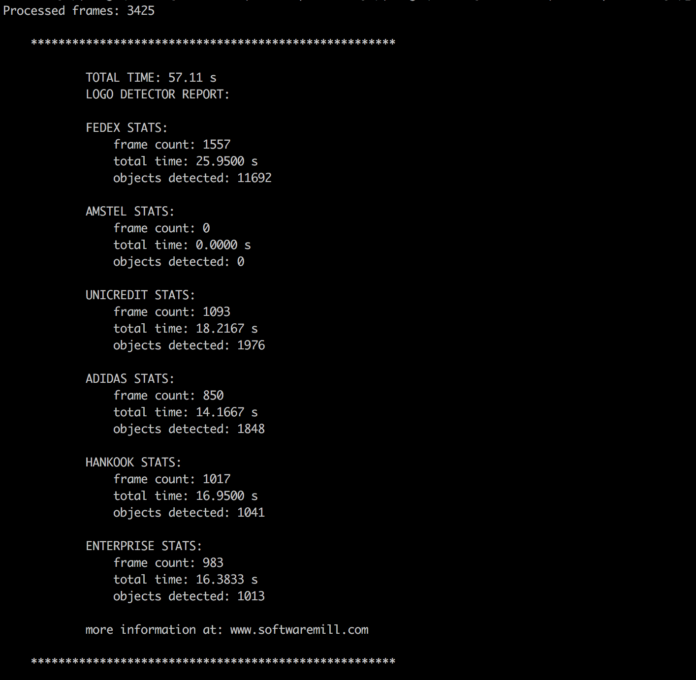
return resultThe result after processing a bit less than 1 minute video from the second half looks like the following:
Additional information:
- All code available at: https://github.com/softwaremill/detectnet-tests
- Software versions used: DIGITS ver. 4.0.0, Caffe: 0.15.9,
- AWS Instance used for training and testing: g2.2xlarge
- GPU: GRID K520